In highly imbalanced datasets, where the number of instances in one class greatly exceeds the number of instances in the other class, machine learning models can have a bias towards the majority class. As a result, the models may not accurately capture the patterns and characteristics of the minority class, and treat it as noise or background information. This can lead to poor performance and inaccurate predictions for the minority class.
In fraud detection, such as credit card applicants prediction models, identifying fraudulent applicants is often critical. However, the data of fraudulent cases, or ‘bad’ applicants, is typically rare in comparison to the number of non-fraudulent cases, or ‘good’ applicants. This results in an imbalanced dataset, which can pose a challenge for machine learning models.
The details of the dataset and modelling can be checked here. The original dataset is from Kaggle dataset.
1. The base rate of the dataset
For the dataset with a base rate of 1.8%, a all negative model will have a very high accuracy of ~98%. (Accuracy = Number of Correct Predictions / Total Number of Predictions)
However, no bad applicants can be captured. 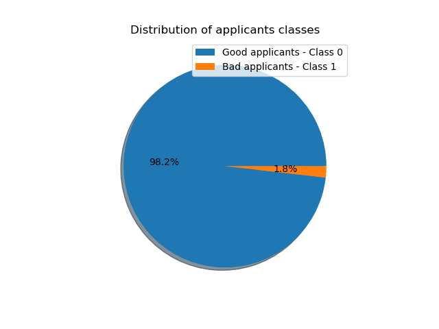
2. Two common methods of dealing with imbalanced dataset
Oversampling of minority class, Undersampling of majority class
Increase the samples of minority class, or reduce samples of majority class. It can help balance the class distribution and improve the performance of the model on the minority class.
SMOTE Synthetic Minority Over-sampling Technique is a popular algorithm to oversample. It works by computing one sample’s k nearest neighbors in the feature space, then generating samples by interpolating between the selected instance and its neighbors.
Weighted classes in models
Assiging different weights to the classes during training, by modifying the loss funcion. This means the loss function will penalize more for misclassifying minority class.
3. Model/methods selection
For the case project, the model and data processing methods highly depend on the specific business value.
Assume that a good applicant will bring some financial profit while a bad applicant will cause financial loss. It is important to calculate the business value in model/methods selection rather than just purely comparing the metrics.
The standards can be simplified as: assume the average profit brought by a good applicant as \(gain\_avg\), and the average financial loss caused by a bad applicant as \(loss\_avg\).
The business value of a model can be represented as: \[TN * gain\_avg - FN * loss\_avg\]
Model selection should be based on comparing business values of different models.
4. Details of different methods handling imbalanced data
More details in this notebook
4.1 SMOTE
# XGBoost with SMOTE
steps = [
         ('over', SMOTE(random_state=1)),
         ('scaler', scaler),
         ('model', XGBClassifier(objective='binary:logistic',
                                 max_depth=5, learning_rate=0.001,
                                 n_estimators=250, reg_lambda=1,
                                 subsample=0.8))
        ]

model = imblearn.Pipeline(steps).fit(X_train, y_train)

ConfusionMatrixDisplay.from_estimator(model, X_test, y_test,
                                      labels = [1, 0],
                                      colorbar=False)
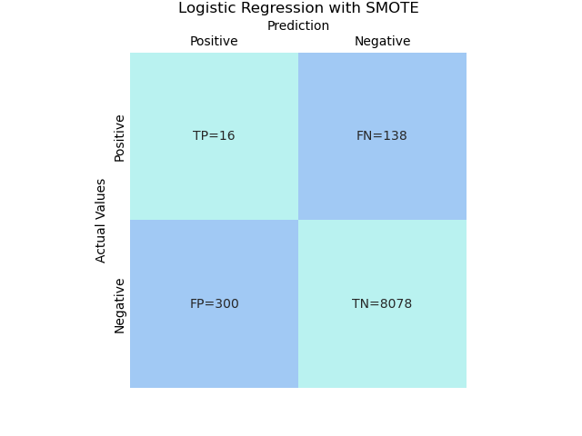
# Logistic Regression with SMOTE
steps = [
         ('over', SMOTE(random_state=1)),
         ('scaler', scaler),
         ('model', LogisticRegression(n_jobs=-1, random_state=1,
                                      max_iter=100000, tol=0.001,
                                      solver='sag', C=0.01))
        ]

model = imblearn.Pipeline(steps).fit(X_train, y_train)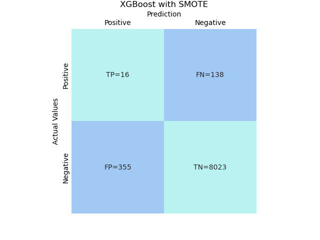
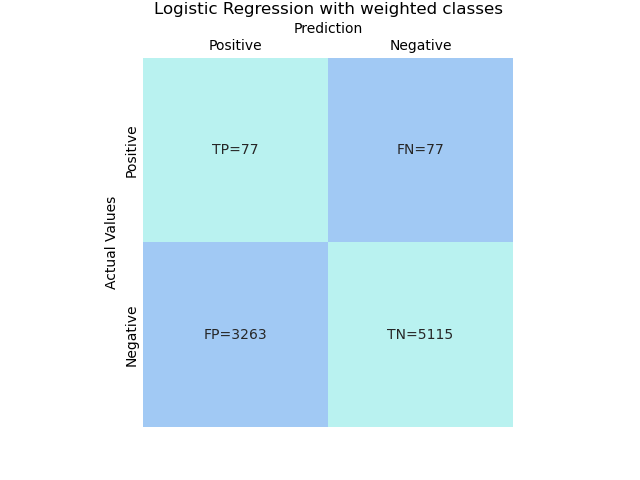
4.2 Weighted classes
# XGBoost with weighted classes
# define the weights by default
scale_pos_weight = y.value_counts()[0]/y.value_counts()[1]

steps = [
         ('scaler', scaler),
         ('model', XGBClassifier(objective='binary:logistic',
                                 max_depth=5, learning_rate=0.001,
                                 n_estimators=250, reg_lambda=1,
                                 subsample=0.8,
                                 scale_pos_weight=scale_pos_weight,
                                 #scale_pos_weight=20 # or define the weights))
        ]

model = sklearn.pipeline.Pipeline(steps).fit(X_train, y_train)
# Logistic Regression with weighted classes
steps = [('scaler', scaler),
('model', LogisticRegression(n_jobs=-1, random_state=1, max_iter=100000, tol=0.001,
#solver='sag', C=0.01,
class_weight='balanced'
#class_weight={1: 30, 0: 1} # or define weights))
]
model = sklearn.pipeline.Pipeline(steps).fit(X_train, y_train)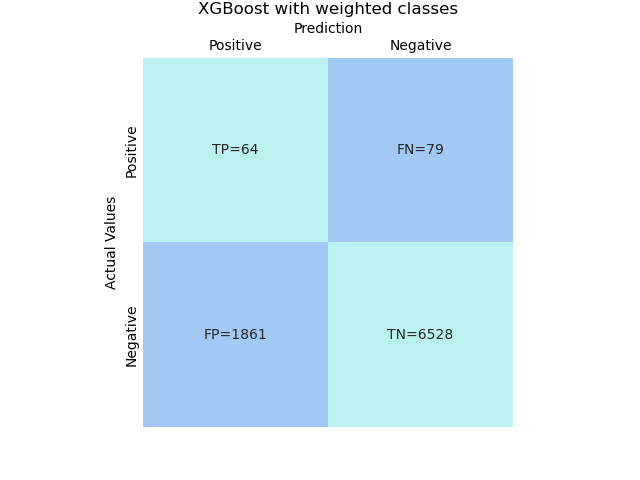
4.3 Weights selection
Tune the number of weights to choose different weights for different business values.
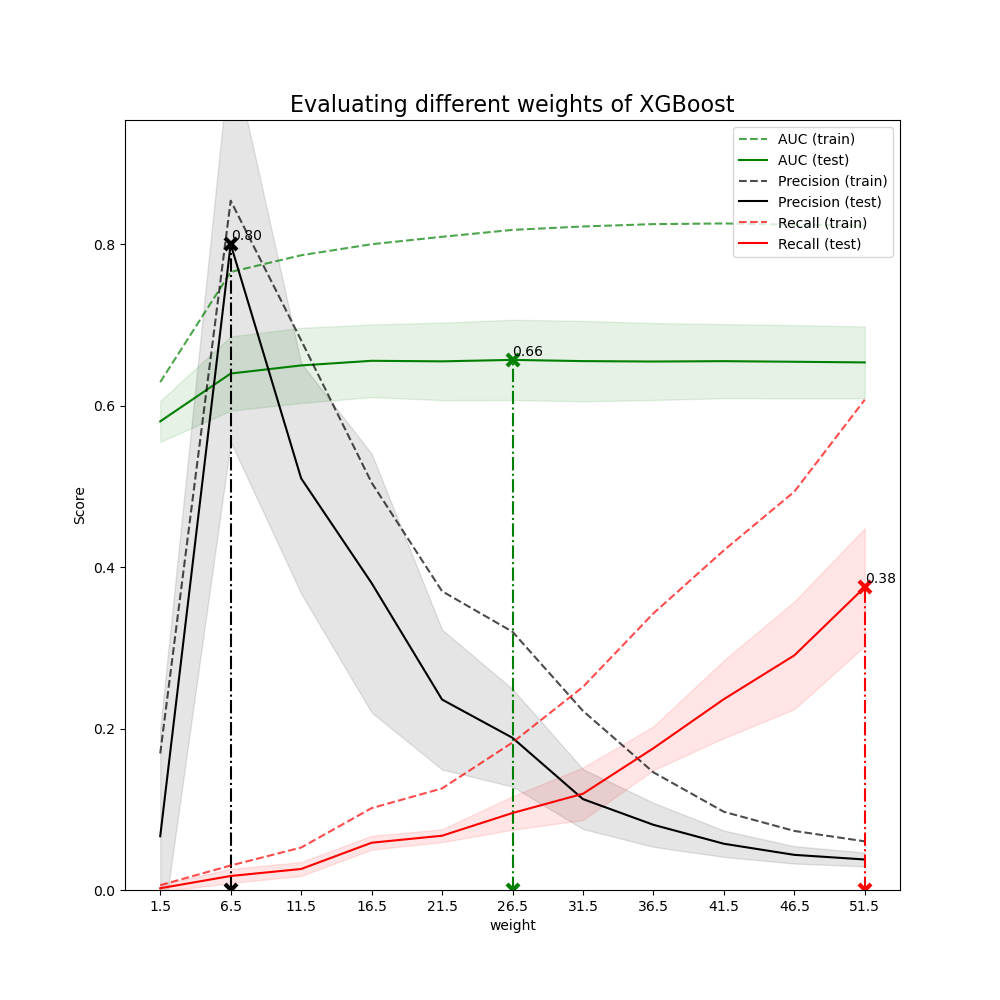
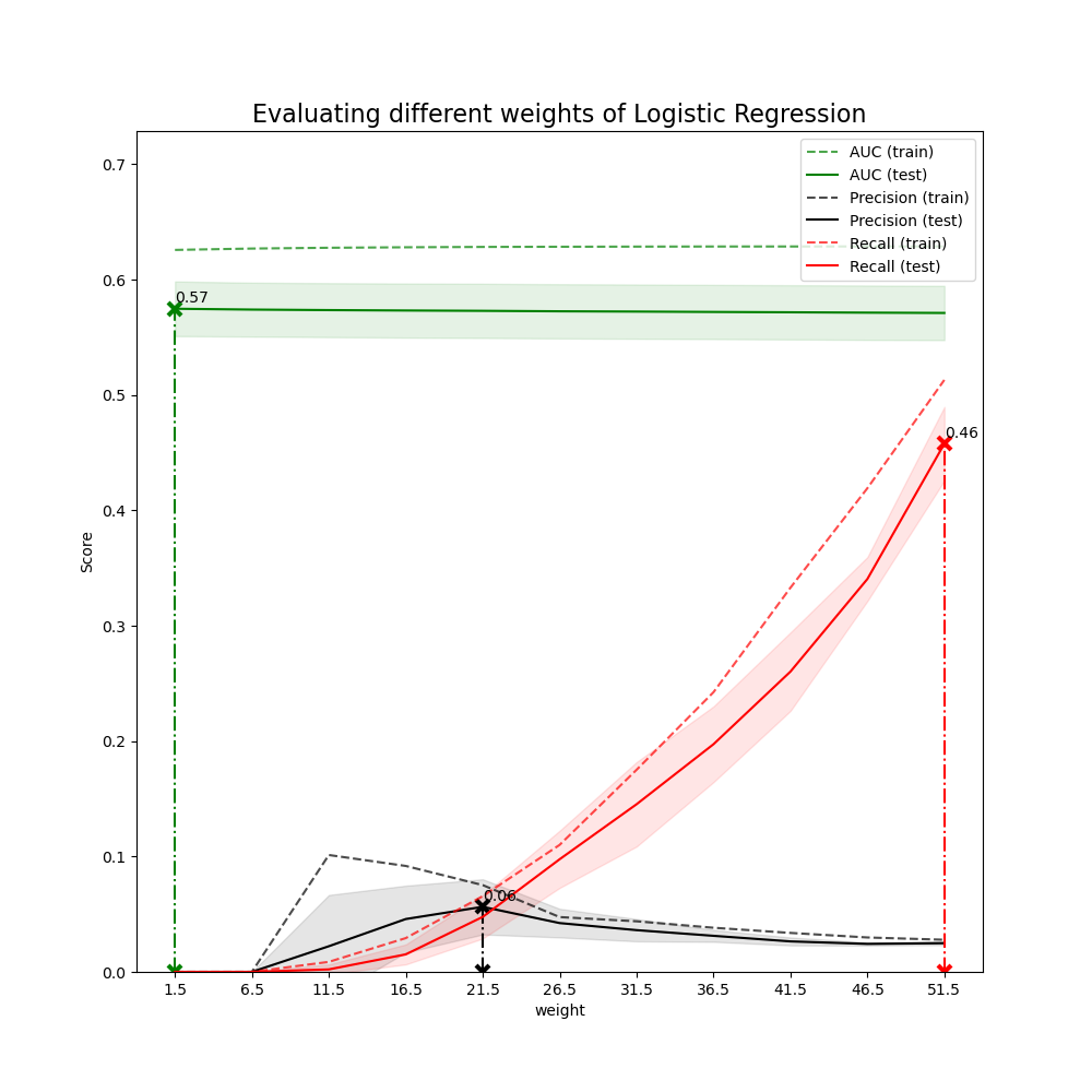
Different weights will change the business values of models
For example, if using weights = 2 in XGBoost, the model shows it will capture 3 bad applicants without any misclassification. The metrics of the model is not good but it will bring more business value compared to no model situation (no bad applicants will be captured).
